Particle Filter

Particle Filter SLAM

Kinematic (실제로봇 위치 이동)

Prediction (가상로봇 위치 이동)

observe (실제로봇과 비콘들 측정)

Add Landmark (측정된 비콘 거리, 각도, ID)

Importance Weight (Particle 오차에 따른 Weight)

Resample (퍼져있는 Particle 모아줌)

Kinematic

Xr : Real Robot position

Prediction

P (.) . Xk : Prediction Robot position

L = 1 : n_particle

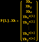
P[L] . Xk = ({{Xk_x}, {Xk_y}, {Xk_θ}, {Yk_x^z[1]}, {Yk_y^z[1]}, {:}, {Yk_x^z[n]}, {Yk_y^z[n]}})

s_dists_rad : noise

각 Particle 에서 noise는 다르기 때문에 Particle이 퍼짐

observe

Real Robot position Xr에서 측정 가능한 Beacon들 간 거리와 각도 z[n] 처리

({{z[n] _dist}, {z[n] _rad}}) = ({{((Beacon[n] _x - Xr_x)^2 + (Beacon[n] _y - Xr_y)^2)^(1/2)}, {atan2 (Beacon[n] _y - Xr_y, Beacon[n] _x - Xr_x) - Xr_θ}})

Add Landmark

측정된 Beacon중 저장된 landmark 중 z[n] 가 없으면 새로 landmark에 추가

P[L] . ({{Yk_x^z[n]}, {Yk_y^z[n]}}) = P[L] . ({{Xk_x}, {Xk_y}}) + ({{z[n] _dist * Cos[z[n] _rad + P[L] . Xk_θ]}, {z[n] _dist * Sin[z[n] _rad + P[L] . Xk_θ]}})

Importance Weight

SSE 갯수는 Particle 갯수와 같음

SSE로 Weight구함

SSE 는 오차이기에 때문에 작은 SSE 값을 큰 weight 값 으로 변환

Wk[L] = Wk[L] * ^(-(4SSE[L])/max[SSE])

Wk[L] = Wk[L]/sum[Wk] : weight  normalize

^(-(4SSE[L])/max[SSE])

[Graphics:HTMLFiles/index_30.gif]

Resample

Wk cdf (Cumulative Distribution Function)

Importance Weight 누적 분포 함수 구한 뒤

오차 분포에서 특정 threshold를 넘의면

다시 오차가  threshold 넘지 않는 것들로 배치 한다 .

퍼져있는 Particle을 모아준다 .

Doc

목적

원리

Goal

x_k : estimate the sequence of hz[n] den parameters

y_k : observed data

p (x_k | y_0, y_1, ..., y_k) : posterior distribution

p (x_0, x_1, ..., x_k | y_0, y_1, ..., y_k) : Markov chain Monte Carlo (MCMC) or importance sampling

sequential Monte Carlo methods (SMC)

Posterior probability

P (θ) : probability distribution function

P (X | θ) : X observation Likelihood

P (θ | X) ∝P (θ) P (X | θ)

posterior probability ∝ prior probability × likelihood

Model

x_k | x_ (k - 1) ~ p_ (x_k | x_ (k - 1)) (x | x_ (k - 1)) : Markov process

y_k | x_ (k - 1) ~ p_ (y | x) (y | x_k)

prediction state space equations

x_k = f (x_ (k - 1)) + w_k

y_k = h (x_k) + v_k

f (.), h (.) : pdf (probability density functions) linear

w_k, v_k : white Gaussian noise

Monte Carlo approximation

sampling - based approaches

 p (x_k | y_0, ..., y_k) : approximate the filtering distribution

P samples expectation

∫f (x_k) p (x_k | y_0, ..., y_k) x_k≈ 1/PUnderoverscript[∑, L = 1, arg3] f (x_k^(L))

Sequential Importance Resampling(SIR)

{(w_k^(L), x_k^(L)) : L∈ {1, ..., P}}

w_k^(L) : importance weights Underoverscript[∑, L = 1, arg3] w_k^(L) = 1

∫f (x_k) p (x_k | y_0, ..., y_k) x_k≈ Underoverscript[∑, L = 1, arg3] w^(L) f (x_k^(L)) : expectation weighted average

π (x_k | x_ (0 : k - 1), y_ (0 : k)) : proposal distribution

π (x_k | x_ (0 : k - 1), y_ (0 : k)) = p (x_k | x_ (k - 1), y_k)

π (x_k | x_ (0 : k - 1), y_ (0 : k)) = p (x_k | x_ (k - 1)) : Importance weight

Step

L = 1, ..., P

x_k^(L) ~ π (x_k | x_ (0 : k - 1)^(L), y_ (0 : k))    : proposal distriution

Overscript[w,^] _k^(L) = w_k^(L) (p (y_k | x_k^(L)) p (x_k^(L) | x_ (k - 1)^(L)) )/(π (x_k^(L) | x_ (0 : k - 1)^(L), y_ (0 : k)) )

π (x_k^(L) | x_ (0 : k - 1)^(L), y_ (0 : k)) = p (x_k^(L) | x_ (k - 1)^(L))

Overscript[w,^] _k^(L) = w_k^(L) p (y_k | x_k^(L))

w_k^(L) = Overscript[w,^] _k^(L)/(Underoverscript[∑, J = 1, arg3] Overscript[w,^] _k^(J)) : normalized importance weights

Overscript[N,^] _eff = 1/(Underoverscript[∑, L = 1, arg3] (w_k^(L))^2) : effective number of particles

Overscript[N,^] _eff<N_ (threshold : Resampling Choose from P)

Probability Density Function

P[a≤X≤b] = ∫_a^bf (x) x

F (x) = ∫_ (-∞)^xf (u) u : cumulative distribution function

f (x) = /xF (x)

cumulative distribution function

F_X (x) = P[X≤x]

F (x) = ∫_ (-∞)^xf (u) u

Probability mass function

f_X (x) = Pr (X = x) = Pr ({s∈S : X (s) = x})

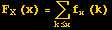
F_X (x) = Underscript[∑, k≤x] f_x (k)

Normal distribution

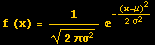
f (x) = 1/(2πσ^2)^(1/2) ^(-(x - μ)^2/(2σ^2))

μ = 0, σ^2 = 1 : Standard normal

Ν (μ, σ^2)

μ∈R - mean

σ^2≥0 - variance

F_X (x) = P[X≤x] = 1/(σ_x (2π)^(1/2)) ∫_ (-∞)^x^(-(k - μ_x)^2/(2σ_x^2)) k = Ν (μ_x, σ_x^2)

Variance σ^2

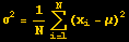
σ^2 = 1/NUnderoverscript[∑, i = 1, arg3] (x_i - μ)^2

μ = 1/NUnderoverscript[∑, i = 1, arg3] x_i

^(-(4SSE[L])/max[SSE])

Plot[^(-4x/100), {x, 0, 100}]